Sunday, November 18, 2012


Chapter P

P.1
 Order Pairs (x,y)
X represents the distance of the point from the Y axis
Y represents the distance of the point from the X axis

Quadrants 

pastedGraphic.pdf

Translating Points

Original Points Transformed Point 

(x,y)     (-x,y)    reflection of the original point in the Y-axis

(x,y) (x,-y)    reflection of the original point in the X-axis

(x,y) (-x,-y)   reflection of the original point through the   origin


Distance Formula 
Given the two points (x1, y1) and (x2, y2), the distance between these points is given by the formula:
  • pastedGraphic_1.pdf

Midpoint Formula
If the coordinates of A and B are ( x1, y1) and ( x2, y2) respectively, then the midpoint, M, of AB is given by the following formula (Midpoint Formula). 

pastedGraphic_2.pdf

Standard Form of the Equation of a Circle 
pastedGraphic_3.pdf
The point (h,k) is the center of the circle, and positive number r is the radius of the circle. The standard form of the equation of a circle whose center is the origin is 
  pastedGraphic_4.pdf
P.2
Determining Solution Points 
The point (2,13) lies on the graph of y = 10x-7 because it is a solution point of the equation 
y = 10x - 7
13 = 10(2) - 7
13 =13
How to Sketch the Graph of an Equation by Point Plotting 
1.If possible, rewrite the equation so that one of the variables is isolated on one side of 
the equation.
  1. Make a table of several solution points.
  2. Plot these points in the coordinate plane.
  3. Connect the points with a smooth curve. 

Using a Graphing Utility to Graph an Equation 
  1. Rewrite the equation so that y is isolated on the left side.
  2. Enter the equation into a graphing utility.
  3. Determine a viewing window that shows all important features of the graph.
  4. Graph the equation. 

P.3
pastedGraphic_5.pdf
Slope
The slope m of the non vertical line 
pastedGraphic_6.pdf
Point - Slope Form
y y1 = m(x x1)
Slope - Intercept Form
y = mx + b
Parallel lines are only parallel if the slopes are equal.
Perpendicular lines are only perpendicular only if the slopes are negative reciprocals. 
P.4
Solving an Equation
2x2 - 5x - 12 = 0.
(2x + 3)(x - 4) = 0.
2x + 3 = 0 or x - 4 = 0.
x = -3/2, or x = 4.
Finding X and Y intercept 
  • y = 0 for the x-intercept(s), so:
  • 25x2 + 4y2 = 9
    25x
    2 + 4(0)2 = 9
    25x
    2 + 0 = 9
    x
    29/25
    x = ± ( 3/5 )
  • x = 0 for the y-intercept(s), so:
  • 25x2 + 4y2 = 9
    25(0)
    2 + 4y2 = 9
    0 + 4y
    2 = 9
    y
    29/4
    y = ± ( 3/2 )
Points of intersection
y = 3x + 2, x = pastedGraphic_7.pdf3 gives
y  =  3(-3) + 2
y  = 
pastedGraphic_8.pdf9 + 2
y  = 
pastedGraphic_9.pdf7
y  =  2x - 1, x = -3 gives
y  =  2(
pastedGraphic_10.pdf3) – 1
y  = 
pastedGraphic_11.pdf6 – 1
y  = 
pastedGraphic_12.pdf7
Thus, the point (pastedGraphic_13.pdf3, pastedGraphic_14.pdf7) is the point of intersection of the two lines. 
Solving quadratics 
Factoring 

  • x2 + 5x + 6 = x2 + 3x + 2x + 6
          = (x
    2 + 3x) + (2x + 6)
          = x(x + 3) + 2(x + 3)

          = (x + 3)(x + 2)
     

Completing the Square 
(x – 4)2 = 5
x – 4 = ± sqrt(5)
x = 4 ± sqrt(5)
x = 4 – sqrt(5)  and  x = 4 + sqrt(5)
Quadratic Formula 

  • pastedGraphic_15.pdf

Solving Equation Absolute Value 
  • Solve | x + 2 | = 7
  • To clear the absolute-value bars, I must split the equation into its two possible two cases, one case for each sign:
  • (x + 2) = 7     or     –(x + 2) = 7
    x + 2 = 7       or     –x – 2 = 7
    x = 5             or     –9 = x
P.5
Solving  Inequalities
7 - 2x < 3
-2x < -4
x > 2
Solving Double Inequalities 
pastedGraphic_16.pdf
Solving Absolute Value 
| 2x + 3 | < 6
–6 < 2x + 3 < 6     
–6 – 3 < 2x + 3 – 3 < 6 – 3
–9 < 2x < 3
–9/2 < x < 3/2

Saturday, November 17, 2012

Rational Functions:


a rational function can be written as


both N(x) and D(x) are polynomials with D(x) not a zero polynomial


The Zeroes of N(x) are the x-intercepts
The zeroes of D(x) are the vertical asymptotes of the function
The degree of the polynomial in the numerator or N(x) over the degree of the polynomial in the denominator or D(x) is where the horizontal asymptote is.

when the denominator has a higher degree the horizontal asymptote is at y=0

when the denominator and numerator have the same degree the leading coefficient of N(x) over the leading coefficient of D(x) is the horizontal asymptote.

When the denominator has less of a degree of the numerator there is a slant asymptote.

ex.


The zeroes of N(x) or 2 and -3 so those are the x intercepts.
The zeroes of D(x) are -4 and 1. These become the places at which there is a vertical asymptote.
The degrees of the numerator and denominator are equal with both polynomials having a leading coefficient of 1 so the horizontal asymptote is 1.

This is what the graph would look like. 


graph_image.aspx.gif

If we were to have the equation 

There would be a hole in the graph at -7 because zero cannot be divided by zero

Good luck reviewing if you need more help visit these links.

Finding vertical asymptotes of rational functions:

http://www.youtube.com/watch?v=_qEOZNPce60

Precalculus Rational functions (holes and asymptotes)
http://www.youtube.com/watch?v=HINeQfh5ZXU


Chapter 4 Review

Radian Measures:

When measuring an angle (either in degrees or radians) you have an initial side and a terminal side. Finding a coterminal angle is when both angles have the SAME terminal side. The figure 1.1 bellow shows what a terminal side it. Figure 1.2 shows an example of a coterminal angle


1.1                                                           1.2

Radian & Degree Conversions:

When converting between radians and degrees we use the formulas:


Examples: 


 To convert degrees to radians; you divide by 180 degrees and multiple by pie. This process allows for the degrees to cancel out, leaving only radians present.

To convert radians to degrees; you divide by pie units and multiple by 180 degrees. This allows for the units of pie to cancel out, leaving only degrees present.

Arc Length:

When wanting to calculate the arch length of a circle we use the formula:


* This equation can only be used when Theta is in radians!!!

Trig Functions (When looking at unit circle):


Trig Functions (When looking at triangles):
Pythagorean Identities:  


Reference Angles: 

As shown bellow in the red, reference angles are the smaller angles that are formed from the terminal side of the original angle. Reference angles allow us to use an easier angle than that of the original angle. When angles are greater than 90 or 180 degrees reference angles are used. 

Graphs of: Sine, Cosine, and Tangent functions:


Phase shifts: 
Adding or subtracting of some degrees inside the the angle, changing the angle causes the whole graph to either shift left (if addition) or right (is subtraction).

Adding or subtracting of some degrees outside of the angle, causes the whole graph to either shift up (is positive) or down (if negative).
  The amplitude of the cosine graph shown is 1. This is due to the fact that each peak and trough is 1 unit from the divider (middle) of the graph. 
   To find the period of the cosine graph we use the equation: 
Graphing sine functions:
   The amplitude of the sine graph bellow is 1. This is due to the fact that each peak and trough is 1 unit from the divider(middle) of the graph, much like the cosine function. 
   To fine the period of the sine graph we use the equation: The same as the cosine graph.
Graphing tangent functions:


Because Tan= sin/cos we are able to determine the tangent graph. The tangent function vertical asymptotes' lay where 'x' intercepts of the cosine function are. We can determine that they are a vertical asymptotes from previous chapters we determined the vertical asymptotes by setting the denominator equal to zero (or when cosine equals zero).
  The period of a tangent function is:

The amplitude of a tangent function is undefined because it is a tangent function.
Graphs of: Sec, Csc, and Cotangent functions:
  
   Graphing cosecant functions:
To graph the cosecant functions you can first look at the graph of the sine function. The cosecant function starts at the peaks and troughs of the sine functions. The csc function has vertical asymptotes when the sine function at the x intercepts. The vertical asymptotes create the csc graph to continue upward and downward towards positive and negative infinity. 

Graphing cotangent functions:
  When graphing cotangent functions you use all the same tools as when you graph tangent functions. the only thing that changes is that the graph will begin to raise on the right to left, instead of left to right.
 Graphing secant functions:
    When graphing secant function you begin the the parent function of a cosine graph. You take all the peaks and troughs on the cosine graph and that is where you begin you secant graph, (at the highest point). The secant graph will have vertical asymptotes where the cosine function crosses the x axis. 

Graphing Inverse functions:

Graphing Inverse Sine functions:
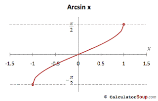
  When graphing an inverse sine function you can only take a small amount of the graph, this is due to the horizontal line test. Because the function doest pass the horizontal line test in the parent function is will not pass the vertical line test unless you cut down part of the graph in the beginning. We want to take the graph of the sine function from negative pie/2 to positive pie/2.


 Graphing Inverse Cosine functions:
    When graphing an inverse cosine function you can only take a small amount of the graph as well. This is also due to the fact that the inverse function wouldn't be fa function because the whole cosine graph is not one to one, only a small part of it is. 
    When graphing the inverse cosine function we want to take from zero to positive pie. 


Graphing Inverse Tangent functions:
    When graphing an inverse tangent function you can only take a small portion of the graph. Like the inverse sine function we will only take a part of the graph from negative pie/2 to positive pie/2. Because he tangent graphs normally have vertical asymptotes they will be horizontal asymptotes once you flip all the x and y coordinates.